AI Demand Forecasting: How It Works, Models, and Cost (2026)
AI demand forecasting applies machine learning models to historical sales data, external signals, and operational context to produce SKU-level demand predictions that are materially more accurate than statistical methods alone. The improvement is most significant for products with high variability, short shelf life, or complex promotional dynamics.
Demand forecasting has been a core supply chain function for decades. What AI changes is the ceiling on accuracy and the handling of complexity. Classical statistical methods (ARIMA, exponential smoothing, Holt-Winters) work well for stable, seasonal patterns with abundant history. They underperform when demand is driven by external signals that do not appear in historical sales data: social trends, weather events, competitor actions, or economic shifts. ML models can incorporate these signals at a scale and speed that statistical methods cannot.
Gartner named AI demand sensing among the core supply chain planning capabilities in its 2026 supply chain technology analysis, noting the shift from periodic planning cycles to continuous sensing and response as AI models replace weekly S&OP reviews with near-real-time demand updates. This guide covers how AI demand forecasting works, the models used, where it outperforms statistics, what it costs, and how to implement in environments with limited data.
For the broader supply chain AI context, see AI supply chain optimization. For the systems that forecasting feeds into, see supply chain management system.
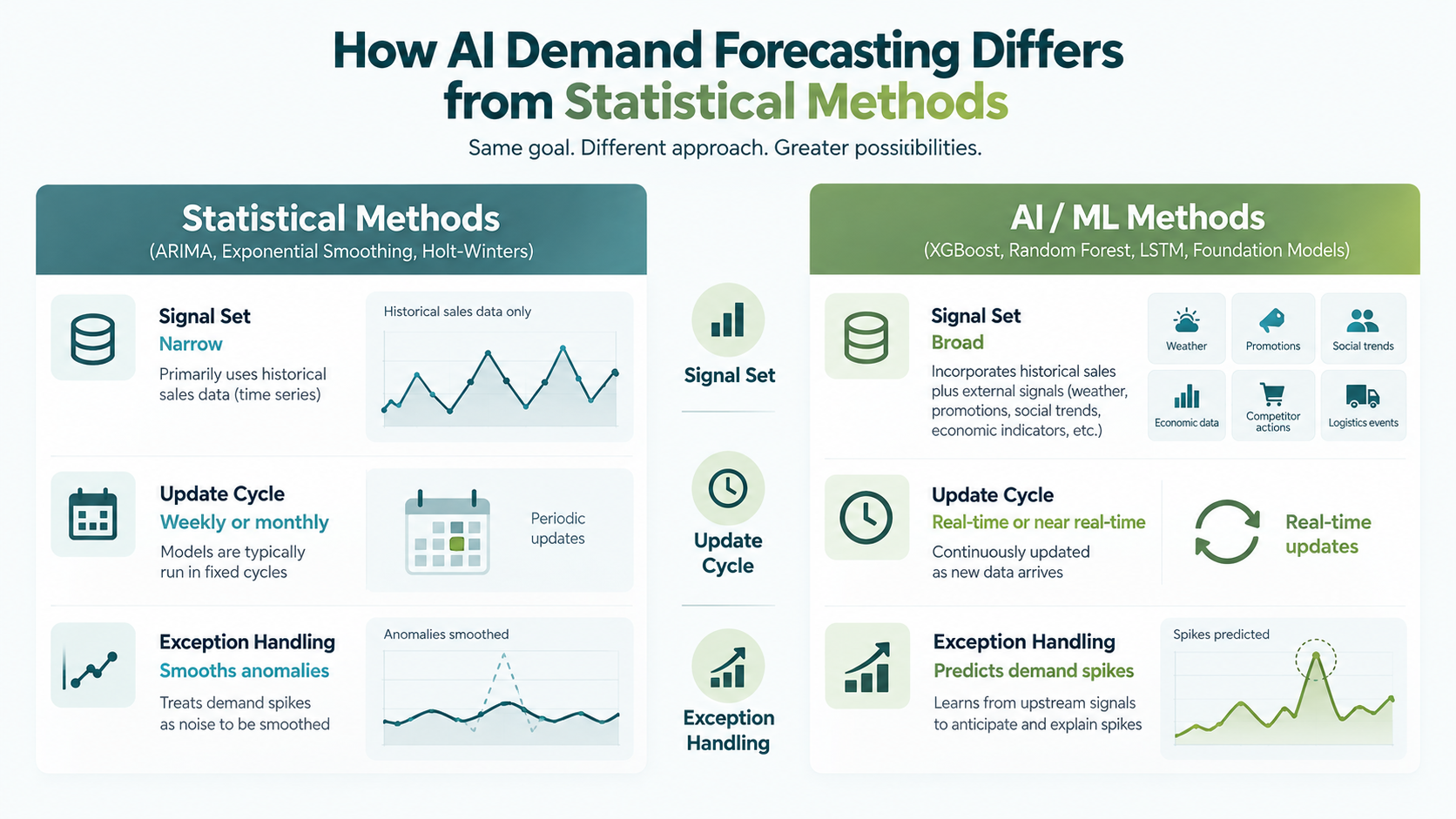
How AI demand forecasting differs from statistical methods: broader signals, faster updates, smarter exception handling
1. How is AI used for demand forecasting?
AI demand forecasting replaces or augments statistical methods by training ML models on historical sales data combined with external signals, producing SKU-level and location-level predictions that update continuously as new data arrives.
The operational difference from statistical forecasting is threefold. First, the signal set is broader. A statistical model uses past sales. An ML model can incorporate weather data, promotional calendars, social media trend signals, economic indicators, competitor price changes, and logistics event data alongside sales history. Second, the update cycle is faster. Statistical models typically run weekly or monthly. ML demand sensing models update in near real time, detecting demand shifts within hours or days rather than the next planning cycle. Third, the exception handling is more intelligent. Statistical models treat demand spikes as anomalies to smooth over. ML models learn to recognize the upstream signals that predict those spikes.
In supply chain practice, AI demand forecasting integrates at the planning layer: the output feeds inventory replenishment decisions, production scheduling, and procurement planning. The accuracy improvement from ML over baseline statistical methods is most consistently documented at 10 to 20 percentage points of MAPE improvement on products with high variability or external signal dependence. For stable, seasonal products with abundant clean history, the improvement is narrower.
2. The four types of demand forecasting
The four types of demand forecasting are passive, active, short-term, and long-term. AI methods apply differently across each type, delivering the most significant accuracy improvement in active and short-term forecasting.
| Type | Definition | Time horizon | Where AI adds most value |
| Passive (intrinsic) | Forecast based on the product’s own historical sales pattern | 1 week – 3 months | Limited: statistical methods competitive for stable patterns |
| Active (extrinsic) | Forecast incorporating external signals: promotions, events, competitor actions | 1 week – 6 months | High: ML handles multi-signal complexity better than statistics |
| Short-term | Operational forecasting for near-term inventory, production, logistics | Days – 12 weeks | High: AI demand sensing detects shifts in near real time |
| Long-term | Strategic forecasting for capacity planning, supplier contracts | 6 months – 5 years | Moderate: AI improves scenario modeling, uncertainty inherent |
3. Which AI model is best for demand forecasting?
There is no single best model. Gradient boosting (XGBoost, LightGBM) leads for structured tabular demand data. LSTM networks lead for time series with long-horizon sequential dependencies. Foundation models and ensemble methods are emerging as the most accurate for complex, multi-product environments.
Gradient boosting (XGBoost, LightGBM)
Most deployedStructured data · High interpretability
The most widely deployed ML approach for demand forecasting on structured retail and supply chain data. Gradient boosting handles tabular feature sets natively: price, promotion flags, weather variables, calendar features, competitor signals, lagged sales. It handles missing data well, trains faster than deep learning alternatives, and is interpretable enough for planning teams to understand which features are driving the forecast. Most demand planning vendors (o9, Blue Yonder, ThroughPut AI) use gradient boosting as a core model layer.
LSTM and transformer models
Deep learningSequential dependencies · High data requirement
Long Short-Term Memory networks model temporal dependencies in sales time series: they learn that demand three weeks ago predicts demand today more than demand 50 weeks ago. Transformer-based models capture longer-range dependencies and have shown accuracy advantages over LSTM for complex, high-frequency demand patterns. Both require more training data and compute than gradient boosting and are harder to interpret, which limits their use in environments where planners need to understand and challenge the forecast.
Foundation models for time series
EmergingZero-shot · Data-light environments
Amazon Chronos, Google TimesFM, and Salesforce Moirai are pre-trained time series foundation models (2024–2025) that can be applied to demand forecasting with minimal fine-tuning, similar to how LLMs are applied to text tasks. They are particularly relevant for data-light environments: when a new product has limited sales history, a pre-trained foundation model generalizes from patterns across thousands of products rather than fitting a model on sparse data. Accuracy benchmarks in 2025 show foundation models competitive with fine-tuned gradient boosting for cold-start and short-history situations.
Ensemble and hybrid approaches
Production standardHighest accuracy · Multi-model
The most accurate production demand forecasting systems typically combine multiple model types: a gradient boosting model for structured signals, an LSTM for temporal pattern capture, and a statistical baseline as a sanity check. The ensemble combines these outputs, weighted by recent accuracy per product and context. This is the architecture used by leading demand planning platforms and reflects the practical reality that no single model dominates across all product categories and demand contexts.
| Model type | Best for | Data requirement | Interpretability | Compute cost |
| Gradient boosting | Structured signals + mixed features | Medium (12+ months) | High | Low |
| LSTM | Sequential time-series dependencies | High (2+ years) | Low | Medium |
| Transformer | Long-range pattern, high frequency | High | Low | High |
| Foundation model | Cold-start, limited history | Low (zero-shot) | Low | Medium |
| Ensemble / hybrid | Production systems, accuracy-critical | High | Medium | Medium |
4. AI-driven forecasting in data-light environments
The assumption that AI demand forecasting requires years of clean, structured sales history is a common barrier to adoption that no longer holds in 2026. Foundation models and transfer learning approaches allow useful forecasting in data-light environments where traditional ML would fail.
McKinsey has consistently documented the challenge of demand forecasting in data-scarce contexts, particularly in emerging markets and for new product launches. The practical approaches that work in low-data environments fall into three categories.
Foundation model zero-shot forecasting
Pre-trained time series models (Chronos, TimesFM) produce reasonable forecasts for new products with no sales history by drawing on patterns learned from millions of time series. Accuracy is lower than a fine-tuned model on an established product but significantly better than a naive baseline. Most practical for new SKU launches, market expansion, or SMBs without historical data.
Analogous product transfer learning
Train the model on products with similar demand characteristics (same category, season, price tier, channel) and transfer learned patterns to the new or sparse product. Works when the portfolio includes established analogues and when the demand driver profile is similar enough to transfer meaningfully.
Synthetic data augmentation
Generate synthetic demand scenarios based on known causal factors (price elasticity estimates, promotional uplift benchmarks, seasonal indices from similar markets) to supplement sparse history. Requires domain knowledge to define the causal model but produces more accurate forecasts than training on sparse real data alone.
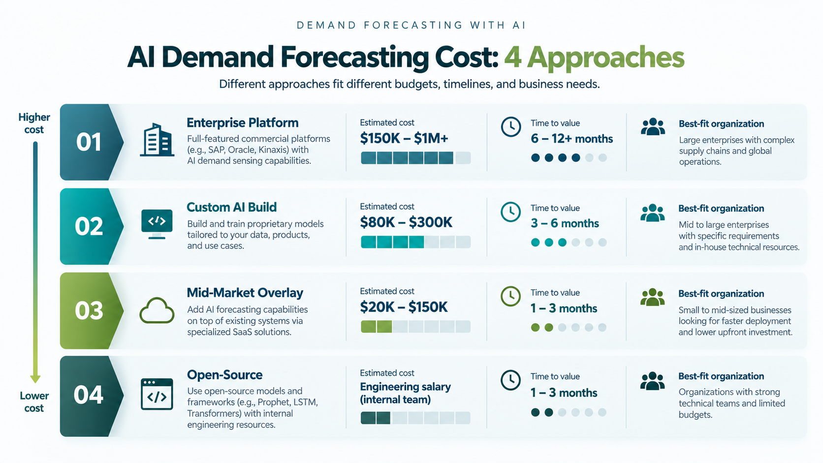
AI demand forecasting cost by approach: enterprise platform, custom build, mid-market overlay, and open-source
5. How much does AI demand forecasting cost?
AI demand forecasting costs range from $25,000 to $500,000 or more depending on whether the organization uses a commercial platform, a mid-market tool, or a custom-built solution. The largest cost driver is not the model but the data infrastructure and integration work.
| Approach | Annual cost range | Time to value | Best for |
| Enterprise platform (o9, Blue Yonder, SAP IBP) | $150K – $1M+ (licensing) | 6 – 18 months | Large enterprise, multi-site, integrated planning |
| Mid-market AI overlay (ThroughPut AI, Streamline) | $20K – $150K/year | 4 – 12 weeks | Mid-market, ERP-connected, accuracy focus |
| Custom AI build | $80K – $300K (build) + $30–80K/yr | 3 – 9 months | Proprietary signals, full control, 3PL product |
| Open-source + internal team | Engineering salary | 6 – 24 months | Technical teams, research, budget-constrained |
6. How to implement AI demand forecasting: the practical sequence
AI demand forecasting implementation follows four steps in sequence: data audit, baseline establishment, model selection and pilot, and production deployment with monitoring. The data audit phase is consistently underestimated and consistently determines whether the project delivers value.
Step 1: Data audit (2–4 weeks)
Map what data exists, where it lives, and how complete it is. Demand forecasting at minimum needs 12 to 24 months of sales history by SKU and location, promotional and pricing metadata, and calendar features. Many organizations discover during this step that data is fragmented across ERP, POS, and spreadsheet systems. Resolving this before model training prevents more expensive discovery mid-project.
Step 2: Baseline measurement (1–2 weeks)
Measure current forecast accuracy (MAPE or WMAPE) by product category and location. This is the baseline against which AI improvement will be measured. Without a pre-deployment baseline, the project cannot demonstrate ROI and cannot secure investment for scale.
Step 3: Pilot on bounded scope (4–12 weeks)
Select a product category with representative demand variability, sufficient history, and a willing planning team. Run AI forecast in parallel with existing method for 4–12 weeks. A pilot that does not improve accuracy by at least 10 percentage points of MAPE versus baseline suggests a data quality or signal selection problem to resolve before scaling.
Step 4: Production deployment and monitoring
Move validated model to production, integrate forecast output into the planning system (ERP, demand planning tool), and establish model monitoring: tracking accuracy degradation over time and triggering retraining when accuracy falls below a defined threshold. Models trained in Q1 often perform less well by Q4; regular retraining is a production requirement.
7. Frequently asked questions
Looking for a Trusted Tech Partner That Delivers Your Measurable Values?
Savvycom builds custom AI forecasting and supply chain analytics systems for operators across APAC, Japan, South Korea, Australia, and the US, including demand sensing pipelines, inventory optimization, and integration with existing ERP and planning infrastructure.
Explore AI and supply chain solutions: Custom Software Development